
Contents
The rest of this article describes some of the most important developments in both methodology and tools that organizations can use to:
Estimating the amount of time and cost required to produce a desired level of certainty, as well as identifying those risks that might be mitigated to make for better results, takes discipline and commitment. There are several key factors resulting in successful risk analysis which we shall explore presently.
This is usually a project schedule with activities loaded with resources that has been reviewed by the team for accuracy in portraying – at least at a summary analysis level – the project plan as it exists. The schedule must also comply with best practice scheduling principles. Good practice critical path method (CPM) scheduling is important since the schedule will be simulated using Monte Carlo simulation methods and specialized software. Simulation ‘computes’ the project many times based on the occurrence of uncertainty and project risks as specified by the project team and others during risk data collection. Using the project schedule facilitates fidelity to the plan. Using resources provides consistent cost and schedule results throughout the simulation.
Project risks represent an uncertain event or condition that, if it occurs, has a positive or negative (opportunity or threat) effect on the activities’ duration and costs, leading, generally, to a later finish date and higher total project cost than planned.
Some analysts collect risk data in workshops, with many people in the room for a day or more. Workshops tend to facilitate discussion and synergy but may not result in data that can be used in the modeling of risks for simulation. There are some pressures characterizing the group risk culture that prevents open and honest discussion and expression of opinion. If present, they jeopardize the quality of the risk data generated and decisions made during group workshops.
Here are a few factors that can negatively affect the quality of group workshop data:
Where members of a cohesive group prefer unanimity and suppress dissent
When an influential person's risk attitude is adopted against the personal preferences of group members.
Making decisions that match the perceived organizational or cultural norms.
Because these pressures impede people’s ability to express their true and honest opinions, an alternative data gathering method – the confidential risk interview – is often preferred. In this interview, people can spend, on average, 2 hours with the risk interviewer, talking in some detail about their views on risk identification and characterization of probability and impact. They do not fear that anything identifiable to them will be told to anyone else.
Often new risks – that are generally not even included in the Risk Register – are identified, even if they are damaging or unpopular “unknown knowns.” Data derived from these interviews is also often more inclusive of key risks and of better quality when people can be free to express themselves, and they only have to commit 2 hours, not a full day or two, away from their project tasks.
An example of a Risk Breakdown Structure (RBS) tool for identifying
project risks at any level of maturity is shown below.

This is the most important precondition of all. With management’s support, success may be achieved in deriving information for decision-makers. If management fails, is disengaged, or is actively trying to manage the message, any and all risk analysis exercises will fail.
Management must support and be seen to enable risk analysis to make its decisions. Management must insist on honesty and realism in the risk data, including requesting “the good, the bad and the ugly” information during interviews or workshops so that all issues can and are discussed honestly and realistically.
Since the platform for cost and schedule risk analysis is usually a resource-loaded project schedule, the software needs to be able to simulate schedules and costs simultaneously.
Today, we have software that handles both uncertainty and project risks. It treats the effect of risks on the cost of labor and of materials differently, as it should. The simulations using modern software produces both cost and schedule risk histograms and scatter diagrams of cost and schedule simultaneously. Current software permits the use of risk drivers as well as discrete risks, and risks can be resolved in parallel or in series. Modern simulation software also automates the prioritization of risks using iterative simulations with a progressive elimination of risks, so management will know the possible days saved if the risk is mitigated.
Uncertainty and identified risks are two distinct factors influencing the variability of results for schedule and cost.
Uncertainty is defined as a background variability, and distinct from the variation caused by identifiable risks. It is caused by at least 3 common factors in projects:
Uncertainty is always present at some level of impact, so its probability is 100%. Since its specific source is not known, uncertainty cannot be mitigated during the time of one project. Uncertainty is applied to all activity durations and resource usage although reference ranges may be used to apply different uncertainty to different phases. The typical expression of uncertainty is in multiplicative terms such as 90%, 105%, and 120%, where the most likely value is expressing a 5% correction for optimistic bias in the durations of the schedule analyzed. The range of uncertainty can differ depending on the type of activity, such as engineering, construction, procurement, or commissioning. Uncertainty is similar to Common Cause in the Six Sigma world and is unlikely to be reduced
Identified risks are root causes of variability that can be measured and potentially moderated or mitigated. These are identified, usually in the Risk Register but also in the confidential risk interviews where we always identify new risks, perhaps those that are unknown knowns. There are generally two types of these risks:
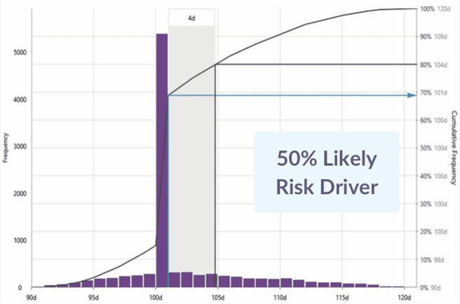
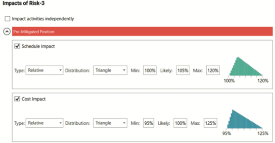
The typical expression of an identified risk using Risk Drivers represents:
Monte Carlo simulation is a way to develop a large, though synthetic, database of projects just like the one under consideration. Monte Carlo simulation is appropriate for solving complex problems, such as project schedules that are not susceptible to mathematical solutions, by conducting multiple trials solving for the finish date or other milestones and total project costs or costs of different project phases to derive statistical statements of the possibility of project finishes.
Statements are of the form: “It is 80% (or some other target of certainty) that the project will finish on this date or earlier, with this cost or less, given the plan and risks we have gathered.” Figures of the results in histograms and cumulative distributions of simulation results are shown later.
The model used is a project schedule, usually developed to WBS level 3 to capture main interfaces but not usually the full detailed contractor’s schedule which omits some work and is often not compliant with best scheduling practices. An analysis schedule can capture all the work at a summary level with less detail than is needed for the daily assignment of work or progressing, and can usually be developed or revised to comply with best scheduling practices. Hence, risk analyses can be done on small-to-medium-sized schedules of 150 – 2,000 activities. The schedule should be reviewed by the contractor and the owner to ensure agreement with both parties that the summary fairly represents the plan at the time of its creation.
Using the project analysis schedule and the risks derived from interviews with project team members ensures that both the platform and the risks are specific to the project. The results for the project’s finish date (and cost) can be interpreted to apply to the project’s prospects.
There are different levels of risk analysis maturity that characterize different project management organizations.
The model below represents risk analysis maturity, not overall project risk management maturity.

Let's explore each of these models and what they represent.
These organizations accept the estimates and schedule results without question. They are ill-prepared and will play fire-fighter whenever project risks occur.
These organizations talk about risk frequently and there may be a ‘risk champion’ who is called upon to respond to risks. They do not follow any method or system, relying on the champion every time. Hence their approach is not organized or repeatable.
This method is probably most appropriate at early project stages before estimates and schedules are available. Risks are identified and sorted by their perceived probability and impact on finish dates, costs, and scope. Impacts are estimated without the benefit of models and the risk probability and impact parameters are assessed in ranges.
Definitions of probability and impact are constructed and used to evaluate each risk. An organizing principle at this level is the definition and application of a consistently-defined set of ranges for risk impacts on objectives. An example of the impact definitions is shown below.

A typical tool at Maturity Level 2 is the probability and impact matrix, an
example of which is shown below.

Since the risks are identified and assessed individually this method at Maturity Level 2, this method cannot provide a viable estimate of total project finish date or project cost. What is produced is typically a Risk Register, which at an early stage can serve to focus on the identified risks facing the project that need to be mitigated (threats) or captured (opportunities).
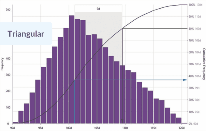
This level uses a project schedule and/or estimate as the platform. A range of low, moderate, and high durations is discovered by interviews or workshops and applied directly to the activities’ durations. A Monte Carlo simulation is conducted, so histograms of finish dates are produced.
However, the individual risks that cause fluctuations are not identified, so cannot be applied to those activities’ durations they affect, including to multiple activities for truly strategic or systemic risks.
Because risks are not used to drive the simulation, nor can individual risks be identified and prioritized for mitigation. The full effect cannot be found of a risk that influences the duration of multiple activities since being placed on activities one at a time. Probability distributions applied directly to the activity duration must incorporate the impact of all risks affecting that activity, so it’s the ‘image’ of those risks, some of which are less than 100% likely, that's projected on the activity durations by distributions such as the triangular distribution below.
At this level, root cause risks are identified, quantified, and modeled against the project schedule. This means that they can affect one, two, or even many activities’ durations depending on the level of generality they represent if they occur during an iteration in the Monte Carlo simulation. Root cause project-specific risks can be assigned to individual activities or phases.
Systemic risks can be assigned to multiple activities including to every activity depending on the effect of weakness in delivery systems that are represented.
Uncertainty is included as a base level of variability that cannot be reduced and is assigned to all activities at Level 4.
The simulation produces histograms and cumulative distributions that indicate the finish dates with probabilities of success – and consequently the amount of time-contingency needed – and are prudent to support contracts and other promises of reliable finishes.
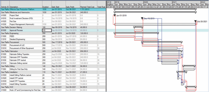
An example summary schedule can be used to illustrate these concepts. The Offshore Gas Production Platform project schedule is shown below:
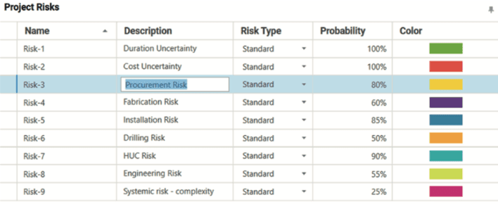
The risks can be identified and quantified with their estimated probability and impact, as shown below.
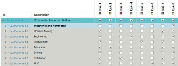
The risks can then be applied to activities or groups of activities as shown below.
The Monte Carlo simulation produces a histogram and a cumulative distribution curve from which statistical results of the modeling can be derived.
For instance, see the schedule risk results below.
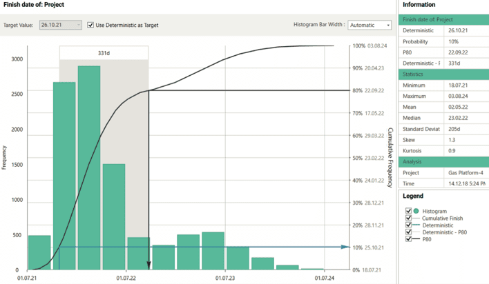
In this case, the results at P-80 show 331 calendar days beyond the scheduled date of October 26, 2021 until September 22, 2022. There's an 80% likelihood of finishing on that date or earlier. It also shows that the deterministic date of October 26 2021 is about 10% likely to be met, 90% likely to be overrun.
These values are before risk mitigation actions are decided and committed. In terms of percent overrun in this case study, from the 1,030 deterministic duration the P-80 adds 32% pre-mitigated. The bimodal distribution is at about 1,600 days or plus 55%, driven by the systemic risk hypothesized as a weak project team given the challenges of this project.
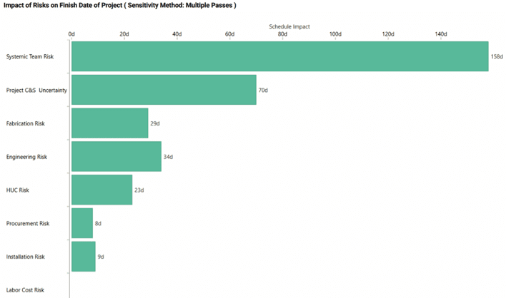
Because the identified root-cause risks (as well as background uncertainty) are driving the simulation, they can be sorted out in priority order at the end of the pre-mitigated simulation results. The payoff for using Risk Drivers to drive the risk analysis includes the opportunity to perform a risk mitigation workshop that develops specific mitigation actions to improve the probabilistic results for a post-mitigation scenario. The best way to prioritize the risks is with an iterative simulation approach that calculates the impact of each risk when it is fully mitigated to the desired level of certainty (e.g. P-80), selecting the most impactful risk by its largest days saved if it were fully mitigated, then simulating all other risks to select the second most impactful risk, and so on.
The best purpose-built software tools have automated this time-consuming effort for fast turnaround. An example of prioritizing, measured at the P-80 level of confidence, is shown below. Notice that the systemic risk, as expected for its seriousness and impact on all activities, is the most important risk to mitigate.
This level of maturity represents the most comprehensive simulation-based risk analysis approach available today for project cost and schedule. All the methods available and strengths performed at Level 4 are available at Level 5. What’s missing at Level 4 is the cost connection. This refers to the impact of schedule duration of activities that are supported by labor and other labor-type resources such as rented equipment. To reflect this cost risk the resources must be distinguished by labor and material types. No further resource detail is needed for risk analysis, though this detail is not sufficient for resource management.
In addition, the costs need to be expressed free of contingency for risk. Typically, cost estimates will have a contingency amount ‘below the line.’ That contingency should not be included in the scheduled at-completion cost to avoid double-counting since the modeling and simulation will re-estimate the cost contingency. (Schedules typically do not have contingency amounts of time added for risk, but if they do have them, these schedule contingency activities should be removed as well.) Contingency embedded in the cost or duration estimates should be eliminated, if possible, again to avoid double-counting.
Both task-dependent and hammock (level of effort) activities’ costs react this way. When the activity or the phase takes longer, it’s logical that the labor-type resources will cost more. The assumption is that the cost of those resources may be proportionate to the increase in duration applied to the average daily expenditure (“burn”) rate.
This relationship between duration and labor cost implies that, for each iteration, the schedule finish and the total cost will be internally consistent, having been driven by uncertainty and those activities that occurred during that iteration.
The integrated cost and schedule risk analysis is shown using the finish date and total project cost scatter diagram.
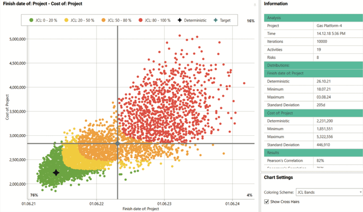
There are other risks that occur to impact cost. Typical cost risks, such as material cost or labor rate variability, may affect cost even if the schedule is perfect. Also, the cost of material resources may vary, especially before procurement and construction contracts are signed. So, cost and schedule are not correlated 100% but are not independent either. This finding is shown in the cost – finish date scatter diagram shown on the previous page.
(The analysis does not presume to determine which party will pay for the added cost of labor or materials, although it is naïve to pretend that a fixed-price contract will effectively shift all cost risk to the contractor. See Merrow conclusion that fixed-price contracts usually define the floor, not the ceiling, of what the owner will pay the contractor.)
The integrated cost and schedule risk analysis is shown using the finish date and total project cost scatter diagram.
That diagram shows a color scheme following ‘JCL’ bands. JCL stands for Joint Confidence Level, which is a name for integrated cost and schedule risk analysis results coined by the US National Aeronautical and Space Administration (NASA) and adopted for their larger projects (over $US 250 million).
There is some analysis of results that show that, since NASA adopted the JCL for their requests to US Congress, their ability to achieve their targets has improved.13 This result doesn’t mean that they’re suddenly better project managers but that when they use Level 5 integrated cost and schedule risk analysis they are better at forecasting where their projects will end up.
Notice that the deterministic plan finish date and cost (each without contingency) provides less than a 20% probability of joint success. As shown by the cross-hairs, the P-80 values for cost and schedule do not, when combine, provide more than a 76% probability of success on both objectives. Obviously, more money and days will be needed to get 80% of the iterations in the south-west quadrant. The amount depends on the degree of correlation between cost and finish date.
The correlation between time and cost is shown at 82%, which is fairly high, so to achieve an 80% probability of hitting both cost and schedule the adjustment to a later date and higher cost will not be extreme.
In order to provide stakeholders with date and cost targets that can both be met with a desired level of confidence, a point on the JCL scatter diagram with that level of confidence for both time and cost should be selected. In general, to the extent that time and cost are not perfectly correlated, the date will be later and the cost greater than those found in the simulation’s histograms and cumulative distributions for time and cost alone.
 Reach Risk Maturity
Discover your organization's level of risk maturity.
