When we talk about the issue of selecting probability distributions for risk quantification in projects, the most popular question is, without doubt, what's the best? Triangular distribution or Pert (also called BetaPert)?
The huge popularity of the Triangular distribution may be because, for many years, it was the only recommendation suggested in PMI's PM-BOK. Any professional certified as PMP had studied Triangular, using it as a useful, convenient, and easy method to incorporate the exPert's criteria by defining its three parameters:
- a minimum value
- a most likely or modal value
- a maximum value
More recent versions of the PM-BOK already include the alternative mention of Pert, but Triangular remains the popular distribution choice in the absence of sample data.
Triangular Distribution vs. Pert
Let's look at an example in project management to clarify which is the best distribution.
In the example of construction of a residence, 8 standard risks have been identified: Risks where, if they were to occur with a certain probability of occurrence, would generate an impact of a certain magnitude, either as a variation in the schedule or cost:
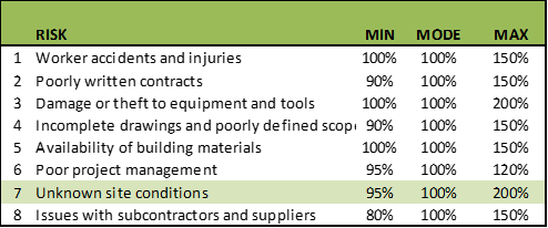
In risk 7, “Unknown site conditions”, a variability of up to 95% of the most probable value is allowed as a minimum point. Concerning the modal value, a reduction of up to 5% in the schedule time or the cost would be expected as a minimum point.
With a maximum value of 200%, this implies that, for the most probable value, the schedule time or cost could be up to twice that value. As seen, there is an asymmetry in the shape of the curve.
There is less variation towards the side of saving time and costs (towards the left or minimum side) than towards the side of extensions in time and costs towards the maximum or right side.
Any experienced project manager knows this is almost always the case. You are more likely to be late than to get ahead of your tasks. You are more likely to go over budget than to underestimate the value of your budget in reality.
See the Pert curve that, using these 3 parameters, could be created for this risk:
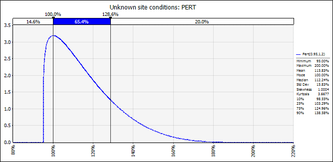
Figure 1
The top of the curve is 100%, the most likely value. The 80th percentile, that is, the point at which 80% of probable events accumulate, reaches 129%. In terms of schedule or cost, there's a 20% probability that the time of tasks impacted by this risk or their budgeted cost, is greater than the respective 129% of the time or modal amount.
Notice what happens if we use these same parameters: 95% of the mode as a minimum and 200% of the mode as a maximum.
But this time, with a Triangular distribution, the cusp of the curve is still 100%, the most probable value. The 80th percentile, the point at which 80% of probable events accumulate, reaches 154%.
So, in terms of schedule or cost, there's a 20% probability that the time of tasks impacted by this risk or their budgeted cost, is greater than the respective 154% of the time or modal amount.
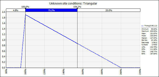
Figure 2
Better still is to compare both distributions:
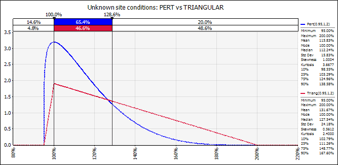
Figure 3
Using the same 3 parameters of minimum, mode and maximum, the Triangular shows a much more conservative scenario. At the level at which Pert maintains 20% of its results above a level of 129%, the 80th Percentile, the Triangular one leaves almost 50% at that level. The area under the curve or probability of results greater than 129% is 20% versus 49%.
That's why we affirm that the Triangular distribution is more skewed, and therefore, it will tend to have tails that are fatter than the Pert, towards the side where the asymmetry is.
As both are asymmetric curves to the right (that is, the right side of both curves carries more probability than the left side), the Triangular one will always tend to carry more probability towards the side of asymmetry; in this case to the right side.
In this example, the Pert distribution has a skewness or asymmetry coefficient of 1.00 while the Triangular one has a coefficient of 0.56.

The Final Impact of Triangle and Pert Distributions
So far, we've not measured the final impact that the choice of one distribution or another has on the results of the project. Let's use Safran Risk to measure such impacts over the activities and the overall project.
In Safran Risk, one first defines the activities on a Gantt type schedule either by creating it from scratch or by importing it from Primavera P6 or MS-Project.
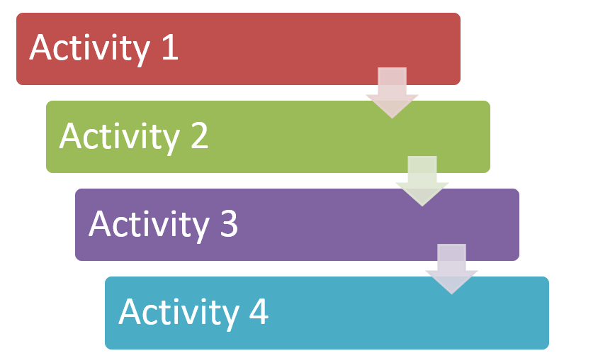
Figure 4
On the other hand, the risks are defined.
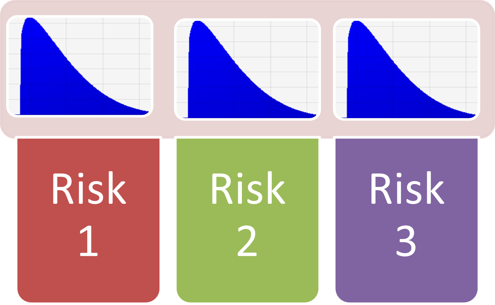
Figure 5
As we have seen in this example, there will be 8 standard risks and we will continue to use risk 7 “Unknown site conditions” for our example:
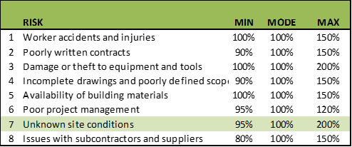
Table 2
Having defined both elements, tasks, or activities and risks, we now proceed to “cross over” which risks impact which tasks in two different dimensions: the duration of the activity and the impact on cost.
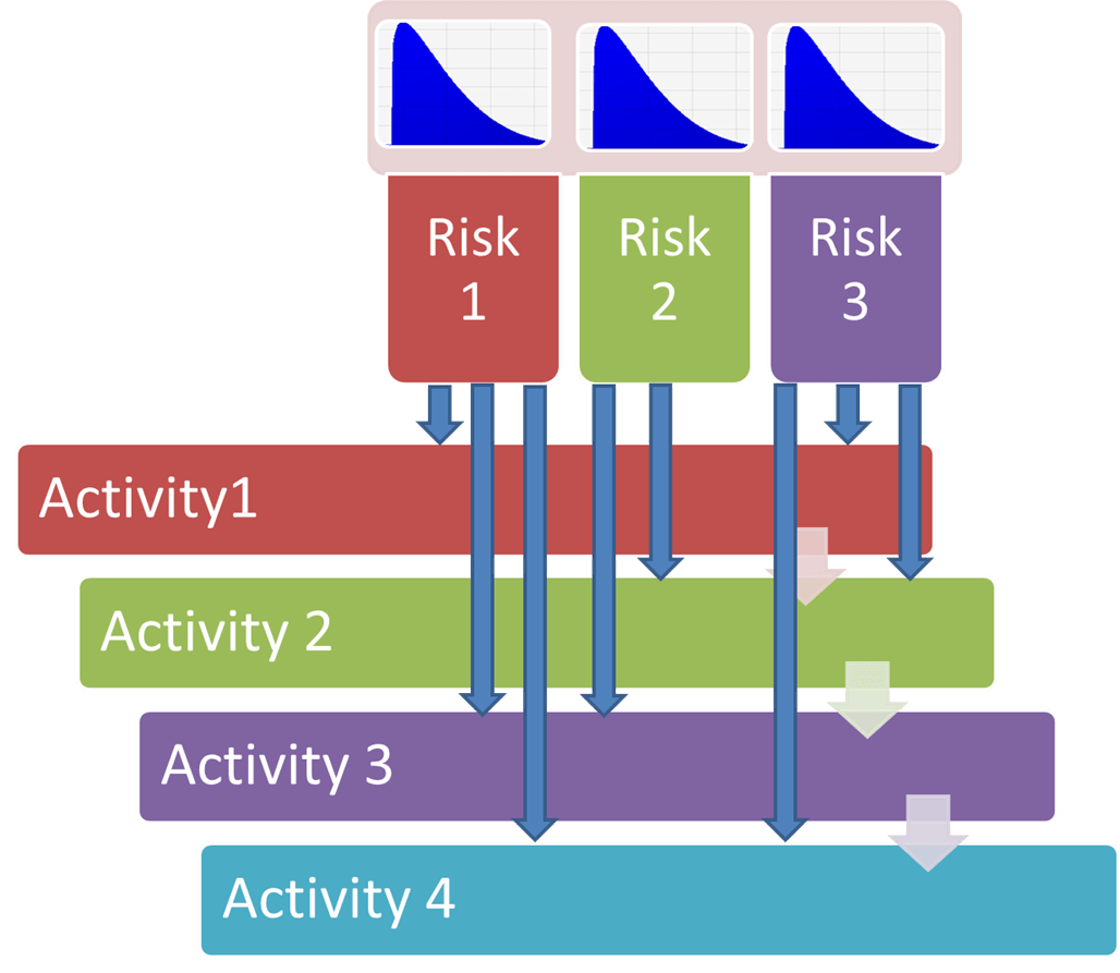
Figure 6
For example, look at Activity 19 “Basement Walls Construction” in Figure 7. It has a deterministic duration of 13 days. In the Risk Mapping tab, you can observe that 3 standard risks impact the duration and cost of this task: “Worker Accidents and Injuries”, “Poorly written contracts” and “Unknown site conditions”.
With the independent interaction of these 3 risks, Safran Risk automatically builds the duration of this task showing the dynamic histogram with a minimum of 11 days to a maximum of 22 days.
Remember the "Unknown Site Conditions" risk is highly asymmetric, and could even double the most likely value in terms of duration and cost.
Let's now run a simulation assuming Pert distributions for all 8 standard risks that impact the duration and cost of project activities.
After simulating, Activity 19 “Basement Walls Construction” would look like this, assuming Pert distributions:
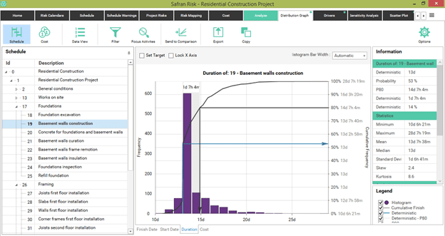
Figure 7
Indeed, the expected value would be 13 days, with a 53% probability of reaching such objective in duration. The 80th percentile would be greater than 14 days, which is 14% longer than expected. This would mean adding just over a contingency day to satisfy an 80% confidence level.
In very extreme conditions, a maximum of more than 28 days could be reached – perhaps when extreme conditions occur simultaneously with the impact of the three risks that affect this activity.
Let's send the duration graph of this task to Graph Comparison to later compare it against the results of an alternative Triangular distribution. We rename this scenario Pert.
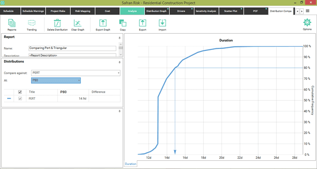
Figure 8
Now, we simulate again but assuming Triangular distributions for all 8 standard risks that have been previously defined. Note that we can implement this in the "Analyze" tab, by using the Pre and Post Mitigation functionality that allows us to evaluate any combination of alternative scenarios.
In this case, we apply all Pert type distributions in the pre-mitigation scenario and all Triangular distributions in the post-mitigation scenario. Previously, for each of the risks, such as "Unknown site conditions", we've added duration and cost impacts with Pert distributions in the pre scenario, and duration and cost impacts with Triangular distributions in the post scenario.
After the respective simulation, we obtain the following results:
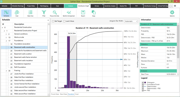
Figure 9
Under these new assumptions, the probability of meeting the deterministic time drops from 53% to 50%, which isn't very significant.
However, the 80th percentile happens to be more than 16 days compared to 14 days under the Pert assumption. This is a 25% contingency concerning the 13-day expected value, compared to the 14% contingency if the assumption of a Pert distribution had been used. While under Pert assumptions the maximum could be 24 days, under the Triangular assumptions, the maximum could exceed 31 days.
By submitting this graph through the Send to Comparison option, we get the following:
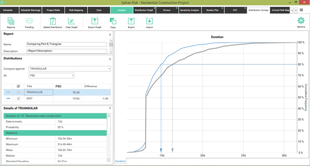
Figure 10
Here it becomes easy to compare the cumulative lines under both assumptions and assess, at P80, how much increase in time contingency would have to be included if the assumption of Triangular distributions were used.
The Bigger Picture
So far, we've seen how, by assuming Triangular distributions, we're being more conservative in assigning higher contingency levels under the same 80% confidence level. Now let's look at what happens in the project in general.
Under the assumption of Triangular distributions, the 80th percentile for the duration of the entire project amounts to 252 days. This is almost 40 days more than its expected value. This is a 19% increase.
In this scenario, there's only a 2% chance of finishing the project before the deterministic duration of 212 days.
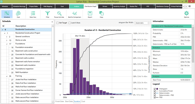
Figure 11
Now, let's see the simulated results, assuming Pert distributions, which we can access by simulating under pre-mitigation conditions.
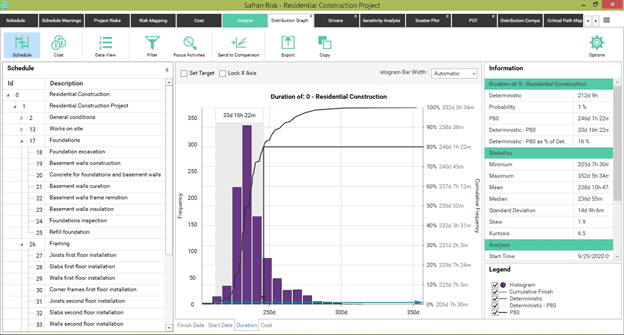
Figure 12
Under the assumption of Pert distributions, the 80th percentile for the duration of the entire project amounts to 246 days.
This is 33 days more than its expected value, a 16% increase. In this scenario, there's a 1% probability of finishing the project before the deterministic duration of 212 days.
By sending this curve through the Send to Comparison functionality, we can compare both assumptions:
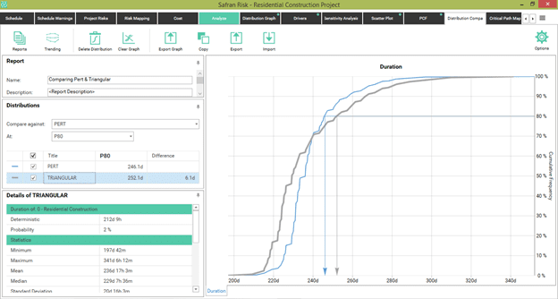
Figure 13
Here, at the P80 level, we observe 6 additional days of contingency required under a Triangular. This is only 2.4% more in the magnitude of such a time contingency. In other words, the final impact on the total project has not been as great as we would've expected, given the differences in the 80th percentiles of the 8 risks considered.
Look at the following table:
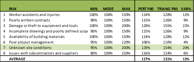
Table 3
In a simple average, the P80s of all the Triangular distributions for the 8 risks are 12% higher than the respective P80s of the Pert distributions.
As we saw in the “Unknown Site Conditions” risk example, the Triangular P80 is 20% higher than the Pert P80. That is, while the Triangular P80 reaches a level of 154% with respect to the modal value, the Pert P80 barely reaches 129%.
How is it then possible that the impact on contingencies, Triangular or Pert, is reduced to only a difference of 2.4% valued at the 80th Percentile level?
The Theory of Conditional Probabilities
The answer has to do with the combinatorial analysis of a Monte Carlo simulation and the theory of conditional probabilities.
With the thousands or tens of thousands of iterations that are generated in a simulation, only in very few cases would high values be simultaneously generated in both one risk and any other in the same iteration. That's because we're analysing a value that is already extreme, which is the 80th percentile.
By definition, the probability that a certain value is exceeded in a certain activity at the 80th percentile is 20%. If you have two activities, the probability of exceeding both simultaneously is not 20% but rather 4% (0.22 = 0.04); since the conditional probabilities are not added or averaged but rather multiplied when there's conditionality or simultaneity.
For this reason, when we compare at the level of an activity, seeing its differences in the tails between one alternative distribution and another; Pert and Triangular, we can observe significant differences.
When we start to add more distributions where some depend in sequence on the others (a project as a sequential series of dependent and simultaneous tasks), and we evaluate a non-central value (such as an 80th percentile), the differences between one distribution and another tend to become less significant. This is due to the compound or power effect that exists in the tails of the distributions.
Triangular Distribution: A Summary
Advantages
- It's relatively easy to specify
- Even if you overestimate the extremes, not significantly at least, it can be considered a conservative distribution.
The Triangular will tend to have tails that are fatter than the Pert ones. The analyst should decide which distribution best describes the behaviour of the tail.
Disadvantages
- In cases where there's a very small possibility of an extreme event, the Triangular will tend to overestimate the probability of an extreme result.
- Triangular assumes the linearity of the probability density function.
We tend to prefer the shape of a Pert distribution, which assumes that the predominance of the results occurs in the most probable range, and then the tails are rounded.
Triangular distribution creates a mathematical discontinuity at its maximum point or mode, something that Pert distribution avoids.
In Conclusion
We can conclude that there's a certain impact of differentiation between the use of Pert and Triangular distributions if the analysis is done at the individual level of activity.
As we add more risks and we see the image from a perspective of the sum of all the tasks in a project, the differences that may exist between one assumption and the other continue to appear. However, these won't be as significant as when they were seen with greater specificity at the level of each activity.
There will be some differences between the use of Pert and Triangular in a project. But in the end, the impact may not be as significant as it would be at the level of each of the activities, in the absence of correlations.
If we were doing this analysis on the averages, there would be arithmetic consistency between the risk variations and the differences between Pert and Triangular distributions because our model has no correlations between risks yet. If correlations were present, the results could be even more or less counterintuitive than they appear to be.
