
One of the key roles a Project Risk Manager plays is helping the team determine how much exposure the project has from the ‘known risks'. This helps them to calculate the amount of cost contingency the project should be retaining.
Normally this has required separate risk models built by risk experts. However, Safran Risk Manager quickly compiles these values for you so that you can forget the complex modelling and focus instead on enhancing opportunity, reducing risk, and making more money on the project.
The Deterministic Approach
In a traditional, deterministic approach to risk management using spreadsheets, the cost risk exposure would have been determined by adding up the factored risk. This means the sum of the likelihood multiplied by the impact of each risk.
If the spreadsheet is a little more sophisticated, then the Post Mitigation values would have been used in this calculation with the anticipation that all treatment strategies would be both implemented and successful.
Based on this calculation, the deterministic cost contingency value would be determined, and this value would be used as the figure for the contingency value in the monthly contract review report.
This approach is simple, cheap and more often than not - wrong. This article will explore why in more detail.

Risk is not a single value
The idea that a project risk can be described as having a 25% likelihood of occurrence and an impact of £100,000 is naive and simplistic. If a risk occurs, then the chances are that it will not be £100,000 exactly, but a value which falls somewhere in the region of £100,000. It will have both a potentially lower value and an upper value which the project team can estimate for (the traditional three-point estimation).
These minimum and maximum values can be thought of as being unlikely to be exceeded. However, the project should not be fooled into thinking that they are the absolute minimum or maximum cost which can befall the project should they occur.
If the spreadsheet has been developed to hold a three-point estimation, which value should be considered the right one for a deterministic calculation? Some calculations would base the value on the most likely, which would then negate the need for a maximum and a minimum.
Other teams adopt “PERT”, an acronym for Project Evaluation and Review Technique, which will apply the formula (O + 4M + P)/6 where O is the optimistic value, M is the most likely, and P is the pessimistic value. This formula provides a weighted average value to the estimate of impact with a greater tendency to the central most likely position, but with a leaning towards either the pessimistic or optimistic side if they are significantly different from the most likely.
On a side note, one additional benefit of the three-point estimation is that it contains sufficient data for the spreadsheet to calculate a degree of confidence in the estimation value. By subtracting the optimistic value from the pessimistic value and dividing by 6, you will obtain an approximation of the standard deviation. The larger the standard deviation, the less confidence there is in the estimation value, and the smaller the deviation range the greater the confidence.
Risk registers and risk exposure are not set in stone
Perhaps the biggest problem with the deterministic approach to assigning contingency values is the fact the risk registers are not static. If they are used correctly, then on a regular basis they should be updated, reviewed, have old risks retired, have impacting risks identified, and have new risks added. This makes for a forever changing picture of what the risk exposure is.
If the budget for the contingency has been set against the deterministic value, then how does the project account for new risks being entered when old risks are not retiring? The project team will identify the new risk to add, see that they cannot simply add it into the register as this will cause the overall value to increase, and so look to see which other risks they can modify either in their likelihood of occurrence, or their impact value.
A few tweaks across the register, and the new risks can slot in nicely without having to declare a contingency increase requirement to the project director.
However, now the project is out of control and probably out of process. It's unlikely that the changes have been communicated to the risk owners, and it's unlikely that a change control record will have been maintained. After a few months of similar changes, the risk register will be so far from the original estimation as to be useless, and a re-base lining exercise will need to be undertaken.
This isn't to say that a deterministic approach isn't valid for some projects types. For instance, a spares or repair contract, where the estimation for spare material or repair effort costs can be determined accurately, parametric values can be used to determine the frequency of occurrence, and a simplified methodology to contingency calculations can be the most cost-effective approach.
If deterministic estimation for complex projects is flawed, then what is the alternative?
Is There a Better Way?
Quantitative Cost Risk Analysis
Quantitative Cost Risk Analysis (QCRA or sometimes just CRA) was developed in the 1950s and 60s by the nuclear industry and NASA as a means of overcoming some of the shortcomings identified, and to bring more of a modelling approach to determining risk exposure.
Building on the concepts of a range of impacts for each risk, a computer model will be built using the risk register data to simulate the potential outcome of each risk within the project given the likelihood that it occurs.
The simulation will run for a number of iterations, usually between 1,000 and 10,000, and this will build a picture of the simulated minimum cost, the simulated maximum cost, and the range of values in between. This is usually visualized using a histogram such as the Cost Histogram. The frequency of a value occurring is on the left hand Y-axis, and the impact value is on the X-axis.
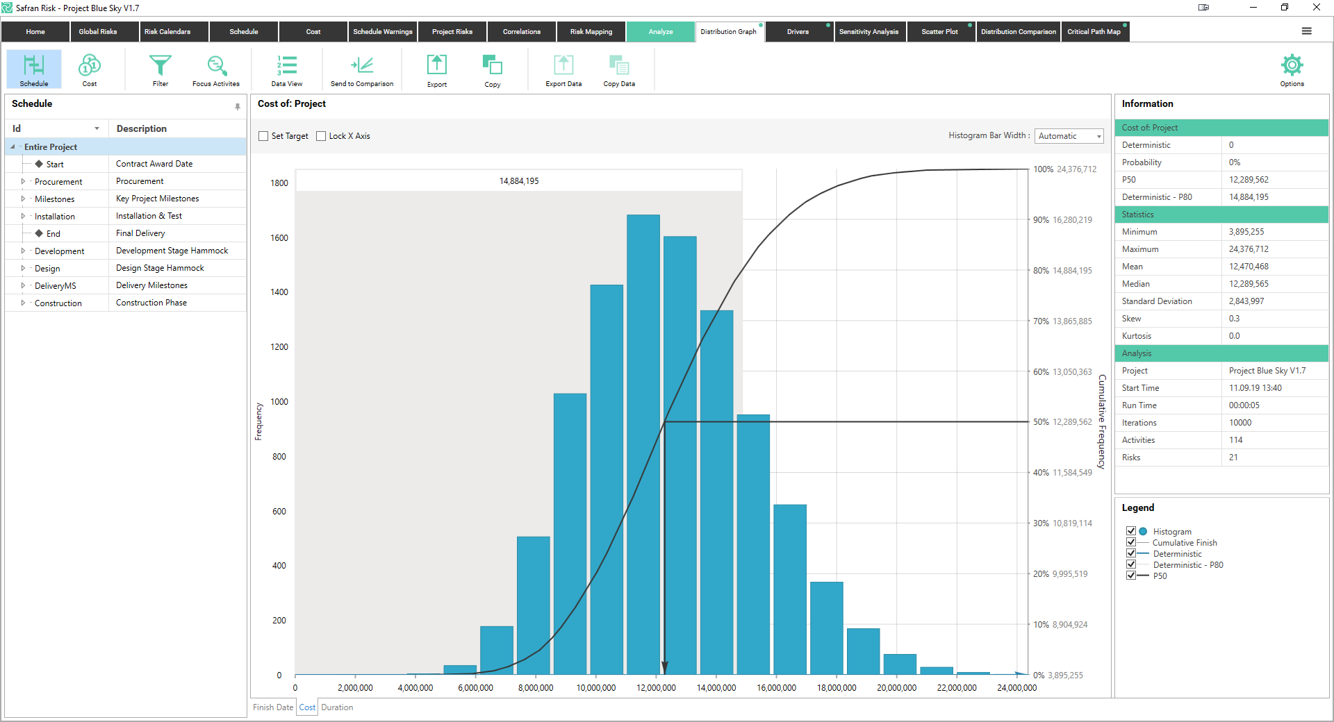
Cost Histogram
In addition to providing useful data about the range of potential cost outcomes of the project, the shape of the histogram can also provide valuable information to the risk analyst. For example, a histogram with a ‘long tail’ to the right of the chart indicates that one or more very high value impacts exist, but that they have a very low likelihood of occurrence.
Sometimes termed the tombstone risks, these risks would quite often be overlooked in a deterministic assessment as the likelihood multiplied by the impact equation produces a small risk value. However, failing to notice this type of risk has the potential to kill the project (hence the name tombstone risk). See the Tombstone Risk Histogram.
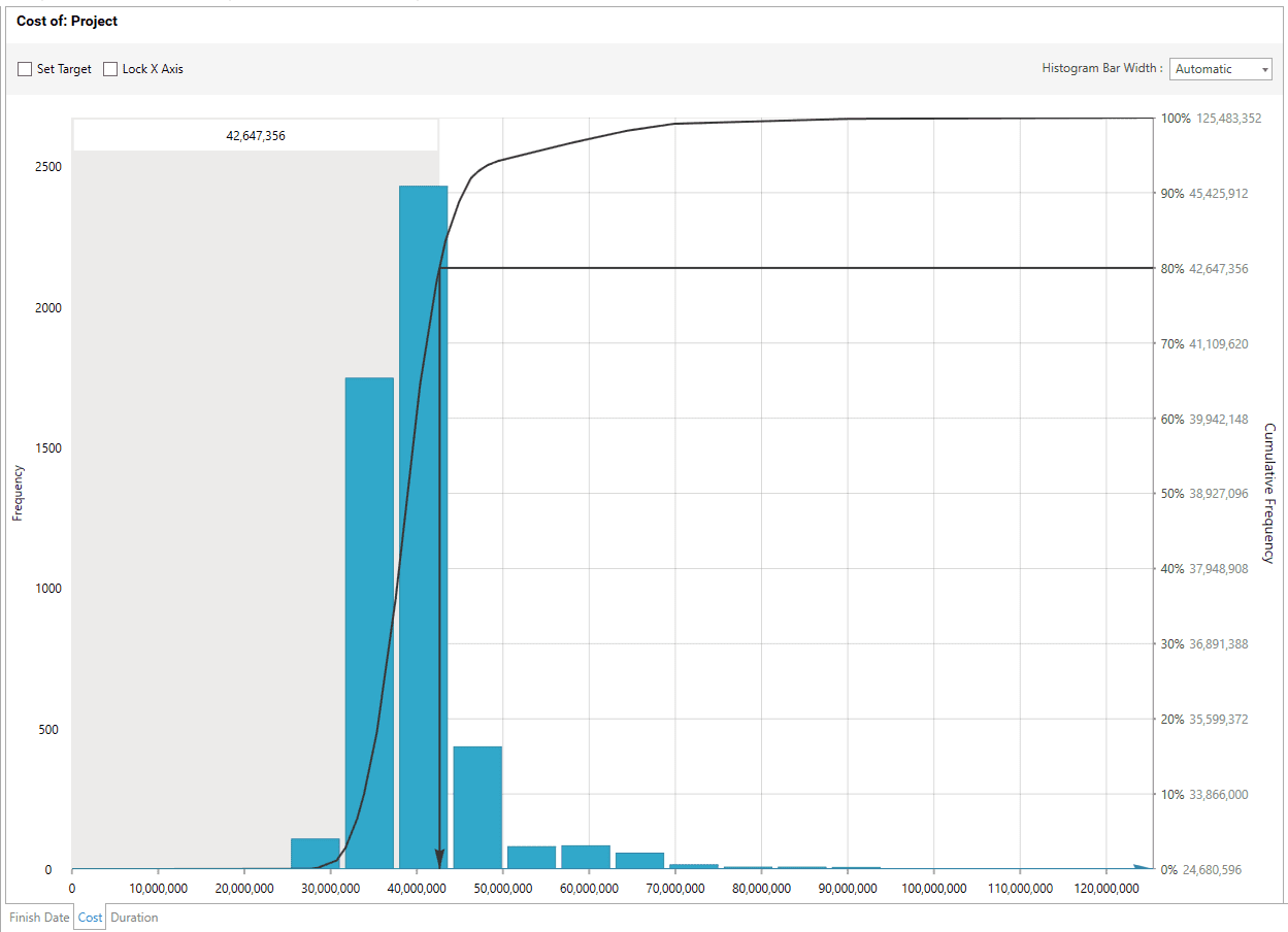
Tombstone Risk Histogram
Another common shape for the histogram is the Double Hump. This shape is characteristic of a risk register which contains a number of evenly distributed impacts but with a few much larger impacts. A common example on a project is when engineering identify the technical risks to a project, but then the procurement team lumps all of the material risks into a single ‘material risk’ line item.
The effect is that the simulation will create the ‘normal’ distribution for the engineering risks, and a ‘single point’ distribution for the procurement risk, which gets combined in the histogram to look like a double hump.
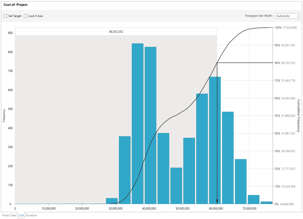
Double Hump Histogram
Determining Confidence
Having computed the distribution of the range of project outcomes, this information can be used to inform the level of confidence which the project has on the achievement of a particular value. To do this, the cumulative distribution curve or ‘S Curve’ is calculated by integrating the histogram data. This ‘S Curve’ is usually overlaid onto the histogram (see the Cost Histogram for a classic ‘S’ shaped curve) and its values are read from the right hand Y-axis usually as a percentage between 0% and 100%.
When reading this axis, it's helpful to use the language which describes the confidence of being higher or lower than a particular value. For example, when describing the confidence of P80 (e.g. the probability of the impact at the 80% probability value) you would say, “There is an 80% confidence that the cost of the project risk will be less than £100,000”.
The alternative view would be to say, “There is a 20% confidence that the cost of the project risk will be greater than £100,000”. It's important to note that the actual likelihood of the project risk cost being exactly £100,000 is zero percent!
Safran Risk Manager
A Model Problem
One argument against the CRA approach is that it requires a high degree of technical understanding of computer modelling in order to create the model in the first place, to generate the histogram and the 'S curve', and then to interpret the results.
Certainly this is true for tools which have separate risk register and analysis capabilities. Safran recognised this difficulty and decided to build a new tool which allows any member of a risk team to identify risks and capture them into an easy to understand risk register.
Once captured, the data then needs to be approved by the project such that the input can be incorporated into the modelling approach. As soon as the approval has been made, the Safran Risk Manager dashboard displays the results of the project model, running 1000 iterations of the simulation.
Now the project team can identify the confidence value around when an assessment of contingency can be made. Note that this is an assessment – the tool will not tell the project team what value of contingency to hold. Instead it will provide the team with various levels of confidence, and the team will need to determine the appetite that the project has for taking risk.
For example, if the project team determines that they will set their risk appetite to 70% of the maximum exposure, then they will set their contingency expectation to not fall below that of the current P70 value. In reality, this means that they will still have a 30% confidence that the cost of risk will exceed the P70 value, and that's the risk they are willing to accept.
Knowing confidence and exposure is a powerful defence
Most project managers will have experienced the occasion, usually towards the end of the financial year, when the finance director is looking to ensure the trading position of the company is as healthy as can be. The low hanging fruit in this situation is to have the projects review their contingency holdings and drop a few percentage points in order to find a good trading position.
Using the deterministic approach, it would be a blind guess as to how much contingency could be released, and the risk register would once again require a tweak here and a fudge there to ensure that the contingency values balanced with the risk register.
By using the modelled exposure positions to determine the contingency requirement against a stated confidence level, it will now be possible for the project team to present a compelling case for appropriate release or prudent retention of contingency.
With a written statement within the project or risk management plan that states, “Contingency will be held above the P70 value for the duration of project phase X”, it's now a very defendable position to say no to the finance director when they demand a contingency release which takes the confidence below the stated position.
The flip side of this argument is that a good finance director would be monitoring contingency holding against confidence positions, and then questioning the team should the values exceed the stated position by a significant degree. This double-edged sword will keep the project managers on their toes, and ensure that a clear and audit-able trail for retention and release of contingency is maintained.
Recording Contingency
Once the project team have identified the contingency value that they are comfortable with against the confidence of project achievement, it would be great if they could track it to better understand how it's being used up, and also how they should prepare for its release in the future.
With Safran Risk Manager, tracking and planning contingency release is straightforward and enables the project team to monitor how contingency is being moved around the project, being used to offset the cost of impacting risks, or being released to margin.
So far we have primarily focused on the contingency of the known risks, for example the risks which are identified in the risk register, which some companies describe as technical contingency or operational reserve. There are other sources of contingency which a project is likely to want to maintain.
These include the management reserve, which is an additional budget out-with of the direct control of the project team and held for the emergence of unknown risks. In addition, some companies will also maintain contingency for penalties or liquidated damages. These contingencies will usually be ring fenced, and only released once contractual clauses have been met.
Safran Risk Manager is capable of maintaining an audit-able trail for any number of contingency types so that the project team can know at any time the total contingency and the split across the different types. Additionally, it also records the transfer of contingency between management reserve and technical contingency, and knows how much is being released to margin, and how much has been consumed by the impact of risks.
Conclusion
Controlling contingency is a vital part of the risk management role and is the most visible aspect of risk management for most organizations during their project control reviews. So, being on top of the contingency and understanding the confidence against the risk exposure is a key tool for the project team to stay on top of.
Through the use of modeling techniques and a high-quality risk management tool like Safran Risk Manager, any project team can be confident that they have their project risks under control.